Have you ever wondered, how the value for exploration data comes to be? What it may depend on? Well...I did. So I have wrote down the values of the scanned planets and stars and looked for dependencies of the payment and the properties of the celestial body. I found, that the payment depends on the mass of the celestial object and want to share my findings with the community.
Stars
Overview
As SVG: View attachment GeneralOverviewStars.svg
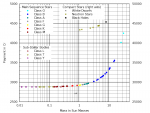
In this figure the payment for different kinds of stars is plotted against the star's mass. In order to show them all in the same graph, two different scaled axes are used. The compact stars refer to the right axis, any other to the left one. There are four distinct groups of stars:
Fitting
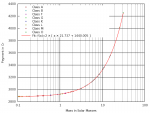
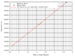
I fitted the main sequence stars as well as the neutron star/black hole data (using Gnuplot 5.0):
As SVG: View attachment MSStars.svg View attachment CompactStars.svg
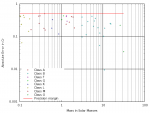
These plots show the data including the fitted function 2*(c*x+b). The factor of two represents the doubling of the payment by using a Detailed Surface Scanner. I have also taken a look into the errors of the fitted function:
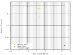
As SVG: View attachment MSStarsError.svg View attachment CompactStarsError.svg
The precision margin is defined by the rounding error of the integer value of the payment. (If the value from the fitted function differs less than 0.5 from the "measured" value, the error will vanish, when the fitted value is rounded to an integer.) As all errors are below the precision margin, the fit is as good as it can be.
Planets
Overview
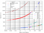
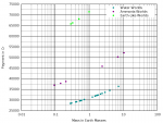
As SVG: View attachment GeneralOverviewPlanets.svg View attachment GeneralOverviewWorlds.svg
These plots show the common types of planets, excluding terraformable variants. This time the mass-dependency is not simply linear. After some trial and error I have found the following correlation between the payment and the mass of a non-terraformable planet:
f(x)=2*[b+c*log2(3)^log10(x)]
with:
Fits
In this section I will present the function shown above fitted to every (group of) planet type(s). As before, the fitted variables will be presented in the graphs and the errors will be shown in a separate graph. The precision margin might start off with a slope. This happens, when the error due to the limited precision of the given mass gets bigger than the integer rounding error. (The planet mass used internally to calculate the value of the exploration data might have been more precise than the value displayed in the system map.)
Low Value Planets
These are the planets with the least value, based on their mass, namely: Icy Worlds, Rocky Ice Worlds, Rocky Worlds and Gas Giants Classes III to V including life bearing ones.
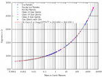
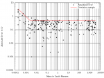
As SVG: View attachment LowValFit.svg View attachment LowValError.svg
Class I Gas Giants
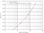
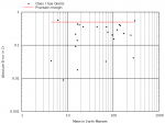
As SVG: View attachment C1GasGiants.svg View attachment C1GasGiantsError.svg
Mid Value Planets
This includes just High Metal Content Worlds and Class II Gas Giants
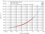
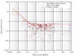
As SVG:View attachment MidValFit.svg View attachment MidValError.svg
Metal Rich Worlds
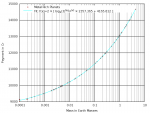
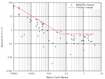
View attachment MetalRichPlanets.svg View attachment mrPlanetsError.svg
Terrestrial Worlds
This includes Water Worlds, Ammonia Worlds and Earth-Like Worlds.
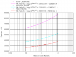
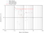
As SVG: View attachment Worlds.svg View attachment WorldsError.svg
Terraformable Planets
They have the same mass-dependency as the planet type they are based upon. The payment for the base type is multiplied by a factor, whose dependency I could not find. I assume, that the factor either depends on a combination of multiple planet properties or that there is a internal "terraformability"-factor, that only loosly or not at all depends on the planets properties. But I can make some statistical assumption, based on my data:
Handout
As it is too time consuming, to use the formula and calculate the value of a planet, every time you have scanned a planet, I have prepared a handout, which might be printed and used to quickly estimate the value of a planet: View attachment HandoutExploration.pdf
I hope I could enlighten the (economical) darkness, that comes with exploration, a bit.
Stars
Overview

As SVG: View attachment GeneralOverviewStars.svg
In this figure the payment for different kinds of stars is plotted against the star's mass. In order to show them all in the same graph, two different scaled axes are used. The compact stars refer to the right axis, any other to the left one. There are four distinct groups of stars:
- Sub-Stellar Bodies: These are the least valuable stars, sticking to 2880 Credits, which seems to be a lower limit.
- Main Sequence Stars: Ranges from 2880 to over 4000 Credits with a linear dependency on the mass.
- White Dwarfs: I have to few data for any statement on their dependency on mass, but they are worth over 25,000 Credits.
- Neutron Stars and Black Holes: Always over 40,000 Credits. They seem to share the same linear dependency on mass, but I don't have enough data on black holes for an empirical statement.
Fitting
I fitted the main sequence stars as well as the neutron star/black hole data (using Gnuplot 5.0):


As SVG: View attachment MSStars.svg View attachment CompactStars.svg
These plots show the data including the fitted function 2*(c*x+b). The factor of two represents the doubling of the payment by using a Detailed Surface Scanner. I have also taken a look into the errors of the fitted function:


As SVG: View attachment MSStarsError.svg View attachment CompactStarsError.svg
The precision margin is defined by the rounding error of the integer value of the payment. (If the value from the fitted function differs less than 0.5 from the "measured" value, the error will vanish, when the fitted value is rounded to an integer.) As all errors are below the precision margin, the fit is as good as it can be.
Planets
Overview


As SVG: View attachment GeneralOverviewPlanets.svg View attachment GeneralOverviewWorlds.svg
These plots show the common types of planets, excluding terraformable variants. This time the mass-dependency is not simply linear. After some trial and error I have found the following correlation between the payment and the mass of a non-terraformable planet:
f(x)=2*[b+c*log2(3)^log10(x)]
with:
- log2(3) being the binary logarithm of 3 (aka the fraktal dimension of the Sierpinski triangle)
- log10(x) being the common logarithm of the planets mass
- c being a coefficient for fitting
- b being a bias for fitting
Fits
In this section I will present the function shown above fitted to every (group of) planet type(s). As before, the fitted variables will be presented in the graphs and the errors will be shown in a separate graph. The precision margin might start off with a slope. This happens, when the error due to the limited precision of the given mass gets bigger than the integer rounding error. (The planet mass used internally to calculate the value of the exploration data might have been more precise than the value displayed in the system map.)
Low Value Planets
These are the planets with the least value, based on their mass, namely: Icy Worlds, Rocky Ice Worlds, Rocky Worlds and Gas Giants Classes III to V including life bearing ones.


As SVG: View attachment LowValFit.svg View attachment LowValError.svg
Class I Gas Giants


As SVG: View attachment C1GasGiants.svg View attachment C1GasGiantsError.svg
Mid Value Planets
This includes just High Metal Content Worlds and Class II Gas Giants


As SVG:View attachment MidValFit.svg View attachment MidValError.svg
Metal Rich Worlds


View attachment MetalRichPlanets.svg View attachment mrPlanetsError.svg
Terrestrial Worlds
This includes Water Worlds, Ammonia Worlds and Earth-Like Worlds.


As SVG: View attachment Worlds.svg View attachment WorldsError.svg
Terraformable Planets
They have the same mass-dependency as the planet type they are based upon. The payment for the base type is multiplied by a factor, whose dependency I could not find. I assume, that the factor either depends on a combination of multiple planet properties or that there is a internal "terraformability"-factor, that only loosly or not at all depends on the planets properties. But I can make some statistical assumption, based on my data:
- High Metal Content Worlds: The factor ranges from 2.5 to 6.7 with a clear tendency towards 6.7. I assume an average factor of around 6.0.
- Water Worlds: The factor ranges from 1.0 to 2.3. I assume an average factor of around 2.0.
Handout
As it is too time consuming, to use the formula and calculate the value of a planet, every time you have scanned a planet, I have prepared a handout, which might be printed and used to quickly estimate the value of a planet: View attachment HandoutExploration.pdf
I hope I could enlighten the (economical) darkness, that comes with exploration, a bit.
Last edited:

